This chapter details the updating required to infer origins and destinations (OD) from automated fare collection (AFC) and other automatically collected data sources provided by the MBTA using the inference software package developed in Gordon (2012). For a detailed explanation of the bus origin-, destination-, and interchange-inference algorithms the reader is invited to refer to that thesis. This chapter will present a high-level overview of the data and algorithms required to perform OD inference and an explanation of the differences between the data available in the MBTA system and in prior work.

This chapter explains the methodology required to generate a month of inferred OD for the MBTA. This includes the data pre-processing methodologies required to synthesize inputs to the OD inference algorithm from AFC, bus AVL, and heavy rail train-tracking data as well as the destination-inference algorithm required for passenger journey stages (equivalent to fare transactions) in the rail network. Additionally, an explanation of modifications made to the interchange-inference algorithm is provided. After a discussion of the validation conducted to test the new methodology, the chapter ends with an explanation of the method used to automate the full inference process so that a month of data could be processed.

Origin Destination Inference Explained

The goals of OD inference is to process data from ADCS to synthesize for every stage, an origin (location and time) and destination (location and time). For networks where transfers can occur unobserved by the AFC system, multiple segments, each on a line, can make up a stage. Some applications have inferred only locations (Zhao, Rahbee, & Wilson, 2007) while others use scheduled trip times to determine arrival times (Nassir, Khani, Lee, Noh, & Hickman, 2011).

The use of boarding and alighting times, as well as the coordinates of origin and destination, are important to journey inference. By applying heuristics to the time a user spends between stages, as well as the spatial characteristics of these stages, one can link stages together into journeys if no trip-generating activity can be inferred to have occurred between stages. In essence, if the primary goal of one stage is to reach the origin of a subsequent stage, then that stage should be linked to the next to form a complete journey.

Open, Closed, and Hybrid Automatic Fare Collection Customer Payment Systems

On the continuum (Figure 2.1) from open to closed AFC payment systems, an open system collects the least amount of information about user behavior: collecting a fee and recording a timestamp only when users enter the system. Examples of this type of system include transit systems in Boston, New York, and Montreal. At the other end of this continuum are closed payment systems, typically with distance-based and/or time-based fares. The calculation of each customer’s fare requires an exit transaction, thus recording the destination location and time such as in Singapore (Robinson, Narayanan, Toh, & Pereira, 2014) or Seoul. Between these two are systems that include a combination of open and closed modes, typically an open bus system and a closed rail system such as in London, San Francisco, and Washington, D.C.

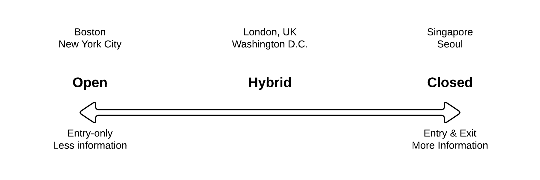
Figure 2.1 Open-Closed AFC Payment Continuum

Generalized Data Flow & Issues

Figure 2.2 shows the generalized flow of the AFC, AVL, and schedule (stop and station coordinates, and stop arrival patterns) data necessary to complete the OD-inference process. The diagram includes only the fields useful to this application, while many others are usually included in each of the referenced tables. The data from some systems can be more processed by design. For example, instead of recording a GPS position and timestamp at given intervals, the London Buses AVL system detects stops along the route and records arrival and departure times. A more recent version of the London Buses AFC system combines AVL and AFC on board to provide an origin location for every transaction, thus bypassing the need for an origin-inference process.

In legacy data collection systems, it is therefore necessary to synthesize automatically collected data prior to origin inference. First one must determine the “pattern,” or the sequence of stops served in a given route and direction, that is being performed by the vehicle. This is done in order to filter the set of stops to which the AVL system GPS records may be matched in order to infer the boarding or alighting stops. By also assigning a pattern to customers, one limits the set of stop events at which the customer can board or alight. This assumes that customers would not stay on a vehicle to travel on its next trip after a terminus. If a set of vehicle-trip start and end times exists then records can be matched to trips temporally, though this requires a reliable time when a vehicle transitions to a subsequent trip.

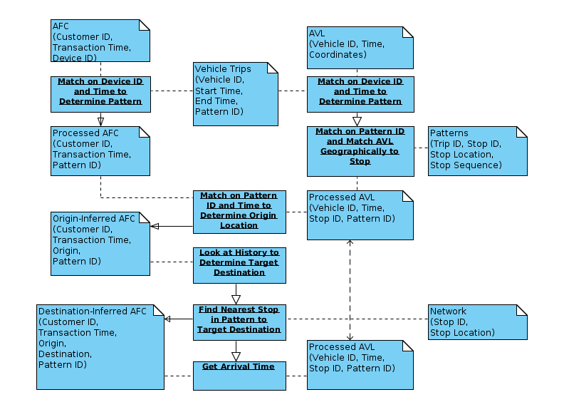
Figure 2.2 Generalized Data Flow for OD Inference, Bolded Boxes Represent Processes, Others Represent Data Sources

In the MBTA context, stop arrival and departure times must be synthesized from raw AVL data and from the set of scheduled stops and their coordinates. Three different methods, depending on available data, are presented in section 2.3.2. With a pattern identified for both vehicle and transaction, and stop events generated, it is then possible to infer an origin by matching the vehicle location to the user based on the transaction time.

By examining a user’s history of transactions and determining their next origin of the day (or the first, presumably home, origin in the case of the last stage of the day), OD-inference algorithms find the information necessary to infer destinations. The method assumes that users do not travel between transit trips via other modes, therefore the destination of the current transaction is assumed to be the nearest stop to the target (often the rider’s next origin, or her first origin of the day) (Barry, Freimer, & Slavin, 2009; Gordon, 2012). Alternatively, for complex and circuitous networks, the destination can be inferred as the stop that minimizes the user’s generalized travel cost (Munizaga & Palma, 2012). The arrival time at that alighting location is determined from AVL and a reasonable set of feasibility checks can be performed to confirm the reliability of the destination.

For rail systems with gated entry, origin times and locations are already recorded in the AFC transaction. The “pattern” used in the rail destination inference is then the network of stations which can be accessed from behind the entry gate. The arrival time can then be inferred from observed stop times at the inferred destination or from scheduled travel times. The methodology for this step is described in section 2.5.3 below.

After origin and destination times and locations have been inferred, interchanges (i.e., transfers) can be inferred by a number of temporal and spatial filters resulting in single or multiple stage journeys being finally inferred.

The Massachusetts Bay Transportation Authority (MBTA)

The MBTA is the transit agency responsible for the operation of bus, light-rail, and heavy-rail transit in the Boston metropolitan area, and oversees the operation of contracted commuter rail and paratransit (see Figure 2.3). Service in the urban core consists of 191 bus routes including four bus rapid transit (BRT) routes, three subway lines, and a light rail line with four branches that operates as a subway in the downtown core. The network includes 7,691 bus stops and a network of 127 light-rail (LRT), heavy-rail, and BRT stations. The average April 2014 weekday has 53,000 stages beginning on LRT, 480,000 on heavy rail, and 341,000 on bus.

Pre-processing Methodologies

The inference of stop-level travel information necessitates greater data accuracy than is typically required for route- or station-level analysis. Transactions that report the bus route but not the vehicle trip, or that include timestamps with a few minutes of error, can be useful for reporting total boardings on a route or in a station during a particular hour. But the origin- and destination-inference algorithms discussed in the previous section require knowledge of the particular vehicle trip, and any temporal error of more than a few seconds can cause the process to choose a different origin stop than the one the passenger actually used. Additionally, and more problematically, a significant enough mismatch between transaction and trip-start times at terminals will infer passengers to be on the wrong vehicle trip, usually travelling in the opposite direction, resulting in the impossibility of correctly inferring origins or destinations for those passengers. This section describes the processing required of each data stream prior to its use within the OD-inference algorithm.

In order to generalize data processing, and reduce the variety of internal data sources to be used, data published in the General Transit Feed Specification (GTFS)[3] and provided online by the MBTA[4] (and many other transit agencies) were used wherever possible. This yielded the scheduled stop times for the modes to be processed, as well as spatial coordinates of these locations.

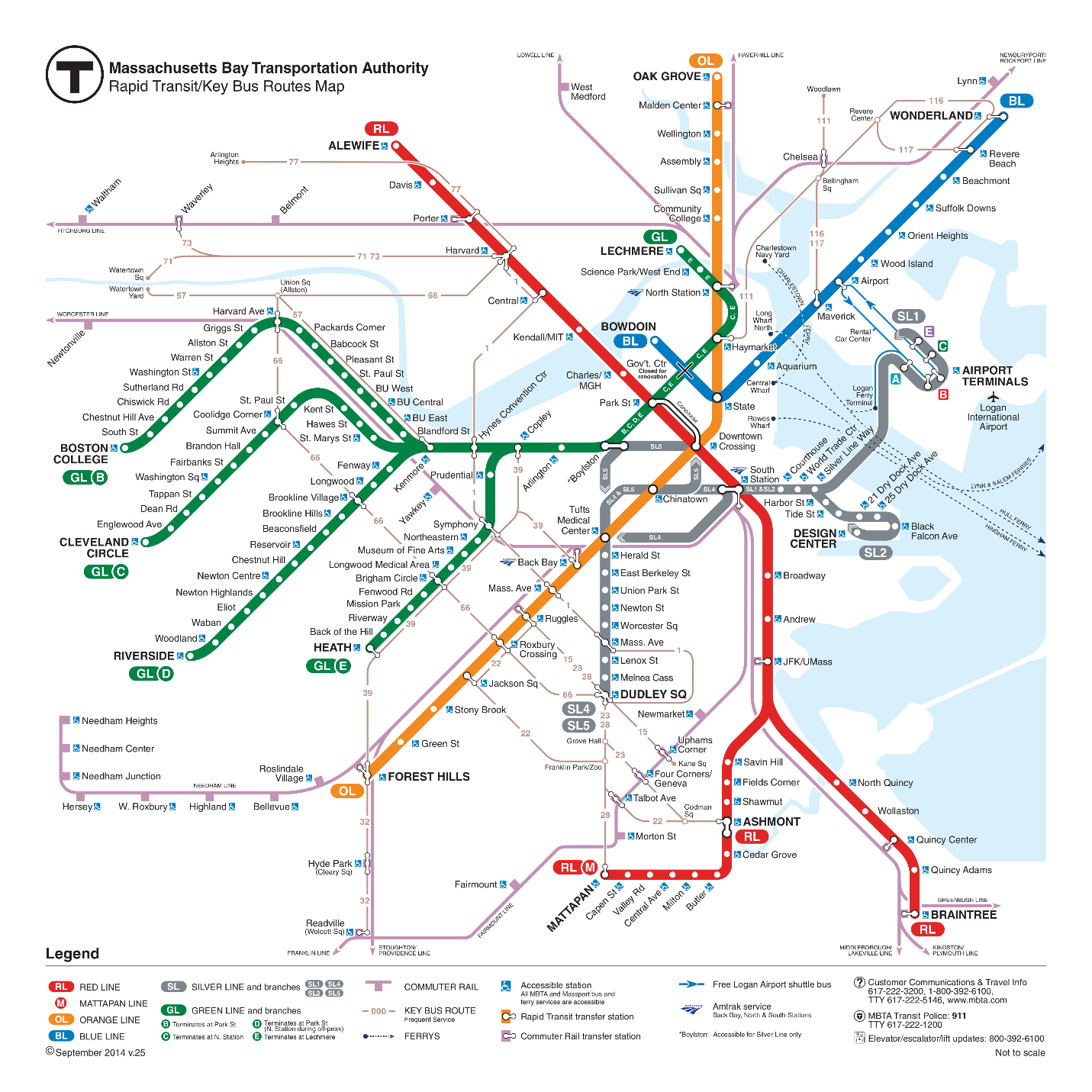
Figure 2.3 MBTA Subway and Key Bus Routes Schematic

AFC

The MBTA’s AFC system collects fares on bus, LRT, and subway. Commuter rail fares are currently validated by conductors and are not recorded automatically, however passes exist that can be used on both commuter rail and the rapid transit network. The AFC system records detailed transaction information for cash, magnetic-stripe paper tickets (Charlie Tickets), and RFID-equipped smart cards (Charlie Cards). Since the AFC table does not contain all of the necessary fields for OD inference, some pre-processing was required. This includes a farebox clock correction algorithm which will be discussed further in the Vehicle Farebox Clock Correction section below. Figure 2.5 shows the entity relational diagram for this preprocessing with the output table on the right (see Figure 2.4 for an explanation of the Crow’s Foot notation relationships between fields in different table).

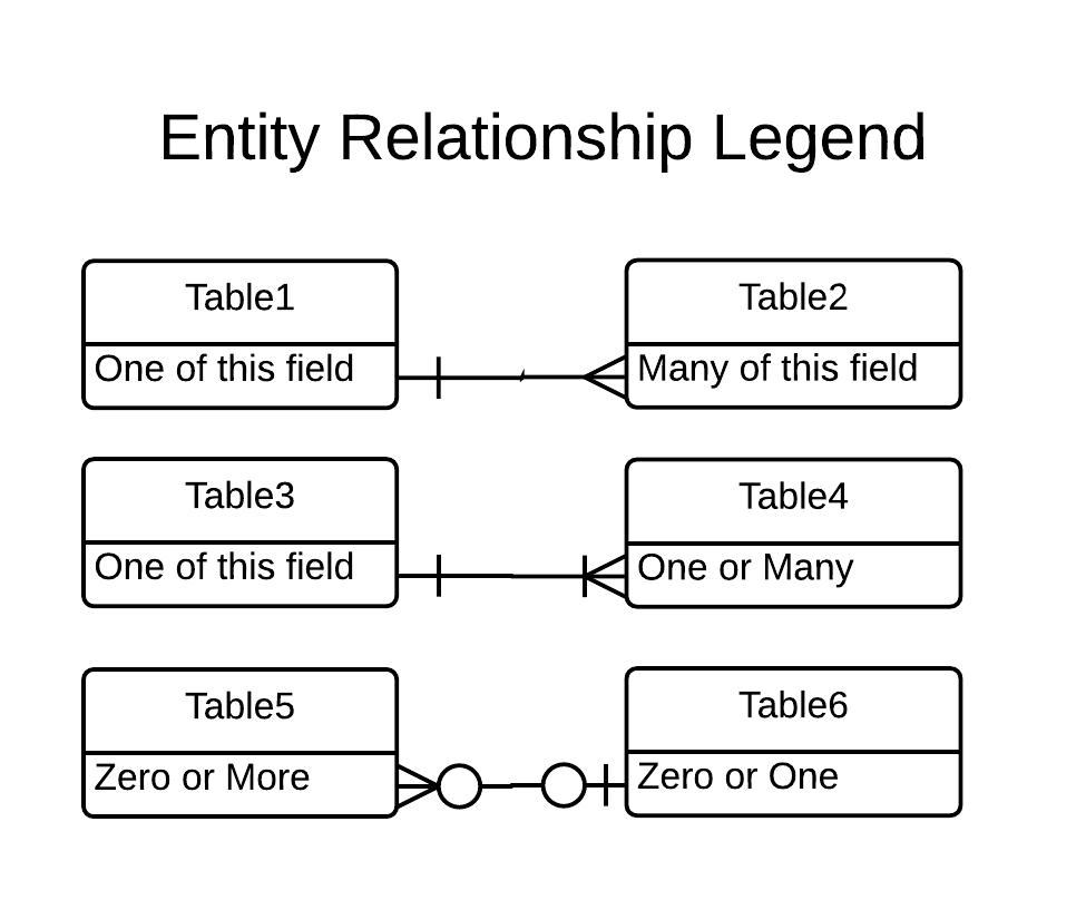
Figure 2.4 Entity Relationship Legend

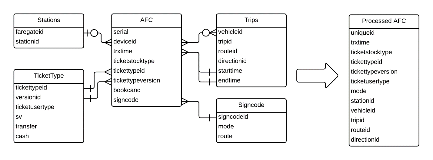
Figure 2.5 AFC Preprocessing Relational Diagram

The goals of the preprocessing are to:

• Create unique identifiers for fare payers
• Assign origins for LRT and other stations
• Assign a mode to every transaction
• Assign a vehicle trip to bus transactions

Unique Identifiers

Because of the mixing of the three payment media (cash, ticket, card), the AFC serial number is not unique across all media and it is therefore necessary to create a compound identifier for users in order to for them to be uniquely identified within the OD inference algorithm. Additionally, transfers are allowed for tickets and cards that pay via stored value, which results in transactions with the same serial number as the original ticket or card, but a different ticket type. Thus, transfer transactions must be linked to the original stored-value ID.

The compound serial is created according to the rules in Table 2.1. Ticket Stock Type is a number which refers to the medium. Ticket User Type refers to the type of discount. Ticket Type refers to the type of pass. A cash serial number is started for every day and incremented with every transaction, so that each cash transaction has a unique ID.

Table 2.1 Unique ID Concatenation Rules

Medium	Fields concatenated
Cash	TicketStockType-TicketUserType-Cash serial number
Ticket (Stored Value or Transfer)	TicketStockType-TicketUserType-Serial
Ticket (Pass)	TicketStockType-TicketType-Serial
Card	TicketStockType-TicketUserType-Serial

Tickets with commuter rail or rapid transit passes are purpose created, so multiple tickets of different types could have the same serial, therefore the ticket type is used to create the unique composite key.

Because cards can have both stored value and passes stored simultaneously, the composite key includes the discount type (TicketUserType) rather than the TicketType.

Assigning Origins to Stations and LRT

By using a look-up table for the deviceid column (the farebox ID) to match to station fare gates, the GTFS station codes are assigned to transactions made at stations. At the time of this writing, the surface portion of the Green Line LRT did not have accurate stop-level AVL data, so origins were inferred at the branch-level on the surface portion of the Green Line. This was done by matching the signcode to a signcode lookup table and using the LRT branch as the origin.

Assign a Mode to Every Transaction

There are three different modes a transaction can have for the purpose of origin inference. The transaction can:

1. be made at a station gate and require its destination to be inferred within the network of stations that can be accessed without making another transaction (all subway, and subterranean LRT & BRT);
2. be made on a vehicle and require its origin to be inferred while requiring its destination to be inferred within the network of stations that can be accessed without making another transaction (surface LRT and select surface BRT);
3. be made on a vehicle and require its origin to be inferred and require its destination to be inferred along a route (bus and surface BRT).

These modes are assigned in the AFC preprocessing using the following mutually exclusive conditional statements, respectively:

1. If the transaction’s farebox ID is matched to a station.
2. If the signcode is a surface LRT or the transaction is assigned to a trip on one of the BRT modes that enters the Silver Line Tunnel (Silver Line Shuttle, Silver Line 1 and Silver Line 2).
3. If the transaction’s farebox ID is matched to a bus and that transaction occurred within a trip.

Assign a trip to bus transactions

In order to limit the set of stops to search for a potential origin or destination for a bus transaction, the transaction is assigned to a bus trip. This is done by matching the transaction to a trip performed by that bus based on the transaction time and the trip’s start and end time. If the transaction happens outside of a trip it is generally assigned to the subsequent trip if it occurred within a reasonable time before the start of that trip.

Vehicle Farebox Clock Correction

After running destination inference, it became apparent that vehicle farebox clocks could run slowly, with potentially inaccurate consequences for origin and destination inference. For example, Figure 2.6 compares inferred boardings and alightings to those observed by the automated passenger counter (APC) system on a bus route that ends at a rail station. The dotted vertical line indicates the temporal boundary between two vehicle trips, and shows that APC system recorded the greatest number of boardings near the beginning of the latter trip. The uncorrected AFC-inferred data show the largest number of boardings suspiciously occurring toward the end of the previous trip.

Further investigation found that clocks are recalibrated when vehicles are in the garage when the farebox communicates with a central server during refueling or cash extraction. In normal operations the clocks will drift, a thorough analysis of all fareboxes revealing that most have clocks drifting by roughly seven seconds per day (Gordon, 2014). Such an error is insignificant for most purposes, but if uncorrected the clock error can lead to inaccuracies in origin and destination inference. This is especially true for transactions occurring at the beginning of a vehicle trip, since, due to clock drift, these will be assigned to the previous trip as in Figure 2.6.

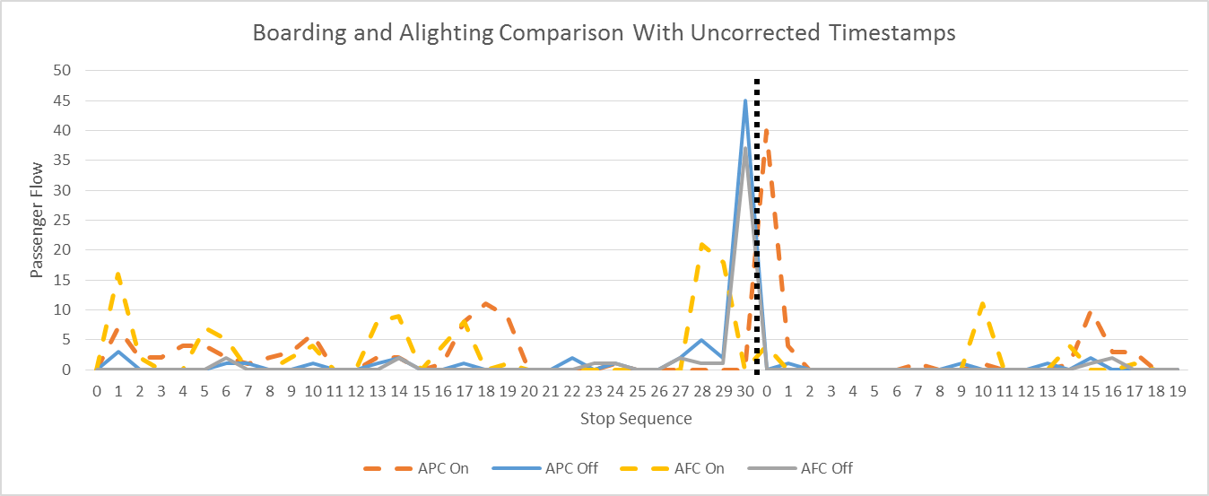
Figure 2.6 Boarding and Alighting Comparison: Uncorrected AFC timestamps

To address the issue of clock drift, the timestamps of AFC records are corrected by interpolating the temporal error of each farebox between clock calibrations. Data from each farebox log, which records the times of clock calibrations and cash removals, are periodically matched to data from that bus’ garage server log, which uses a reliable clock and also records cash removals. Immediately before clock calibration, the connection between garage server and farebox is logged in both databases. Clock correction is performed using the following methodology:

1. The temporal error between the two systems’ observation of this event is determined to be the farebox clock drift since the previous clock calibration.
2. An automated linear regression analysis is performed for each farebox with clock drift as the dependent variable and the independent variable the amount of time since the previous calibration.
3. For each regression, the slope of the regression line, the rate of drift per day, will be used to estimate each farebox’s drift for each transaction using that farebox’s rate of drift and the time since the previous calibration
4. If the regression for a given farebox has too small a sample or too low a coefficient of determination (r²), the median rate of drift from valid regressions is used.
5. Finally, the time of each fare transaction is corrected using Equation 2.1, by adding the product of the time since the device’s most recent calibration and the estimated drift per day.

Equation 2.1

$$\[Corrected\ Time\ = \ Uncorrected\ Time\ + (Time\ Since\ Last\ Probing\ *\ Drift\ Rate)\]$$

This process was automated to correct all transactions. Figure 2.7 shows the result of this correction for the example appearing Figure 2.6. The reader can see that the orange and yellow dotted lines, representing the total boardings estimated using APC and AFC respectively, are much more closely aligned

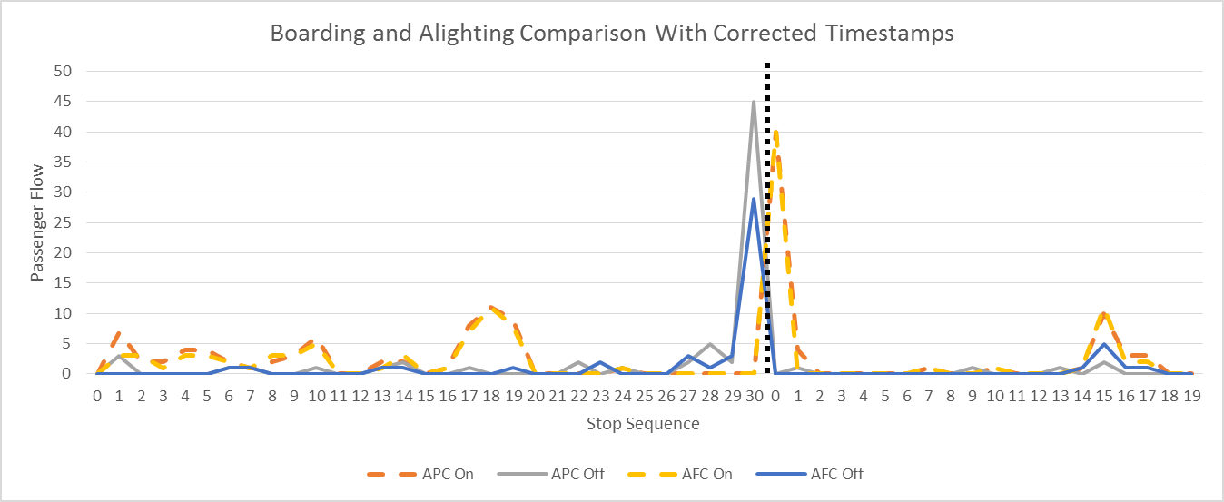
Figure 2.7 Boarding and Alighting Comparison: Corrected AFC timestamps

Bus Stop Events

Unlike in London, the MBTA’s AVL system was not designed to record arrival or departure time at every scheduled stop. Instead the AVL system records timepoints: key stops along a route that are used for performance measurement. Timepoints exist for a median of one in 4.25 stops, with recorded timestamps for one in 4.5 stops.

Interpolation between Timepoints

Using the travel times between stops derived from the GTFS StopTimes schedule it is possible to interpolate arrival times for stops between timepoints. A table of distances between stops was provided, and distances were measured either by odometer or from maps. It would be possible, however, to use GIS to “snap” stops to GTFS shapes and to calculate distances between successive stops, as timepoints have a key which references stops in GTFS.

Interpolation was performed using a custom Java application, which excludes timepoints that are not stops (such as pull-out or pull-in locations or toll facilities), and which handles the 6 percent of timepoints that do not include temporal observations. The interpolator process loops over the timepoint array and searches for timepoint i in the stop array based on stop ID. It then searches for the timepoint i + 1 and sums the distance between the two timepoints. Travel time is calculated as the difference between the departure time of the current timepoint and the arrival time of the next. The time of a given stop event is then linearly interpolated using the average speed between its bounding timepoints and the distance travelled from the previous stop. No dwell time was assumed at stops since the origin inference algorithm was designed to handle only cases where there is only one time observed at a stop.

Announcements

Boston’s buses are equipped with a computer that logs a variety of events with a GPS position, an odometer reading, and a timestamp. In order to comply with the Americans with Disabilities Act (ADA), buses broadcast audio announcements to provide equal access to real- time information for those who are visually impaired. This data set is similar to the AVL in Chicago (Zhao et al., 2007); however, GPS coordinates are included for every logged record.

Internal announcements alert users to upcoming stops and are generally made twice: announcing the next stop when the bus passes through a specified geographic boundary (geofence) around the stop from which it is departing, and again upon entering a geofence around the stop it is announcing. External announcements are triggered by the doors opening and announce the information available on the headsign: the route, direction, and destination.

Internal Announcements

Using internal tables it was possible to associate the text announced by the AVL system with its associated stop. By selecting the last announcement recorded for each stop one could derive a rough approximation of the time at which a bus approached a stop. However, due to the large number of small cities and towns coexisting in the metropolitan area, it is possible for bus routes to have more than one stop with the same name, as stops are not uniquely named for each city. Further, data reliability issues led to the disqualification of this data set as a unique source of information: geofences around stops, like those around timepoints, could be unreliable, and if a bus’s computer was set to the incorrect route (or was suffering other technical difficulties) false positives could be obtained.

External Announcements

There are fewer situations in which no data are recorded for external announcements, as timestamps and GPS positions are still recorded despite some computer errors. Events are triggered and logged by door openings even if the audio is silent because the bus is out of service. The processing algorithm was written and executed in an open-source relational database with a GIS extension, and is executed as follows (see Figure 2.8):

1. The GTFS stop arrivals table includes the stop pattern for every trip. A subset of this table is loaded into a temporary table with the cumulative distance for each scheduled stop calculated based on the either internally measured bus stop distances or distances calculated using the GIS extension. This table is joined to a PostGIS table of the geographic point objects for every bus stop based on stop ID. The locations of bus garages, bus garages with special identifiers populating the route and trip fields are added to this table in order to identify when buses are closer to a garage than to a stop on their route. To improve performance, a spatial index is created and analyzed on the positions of the stops.
   
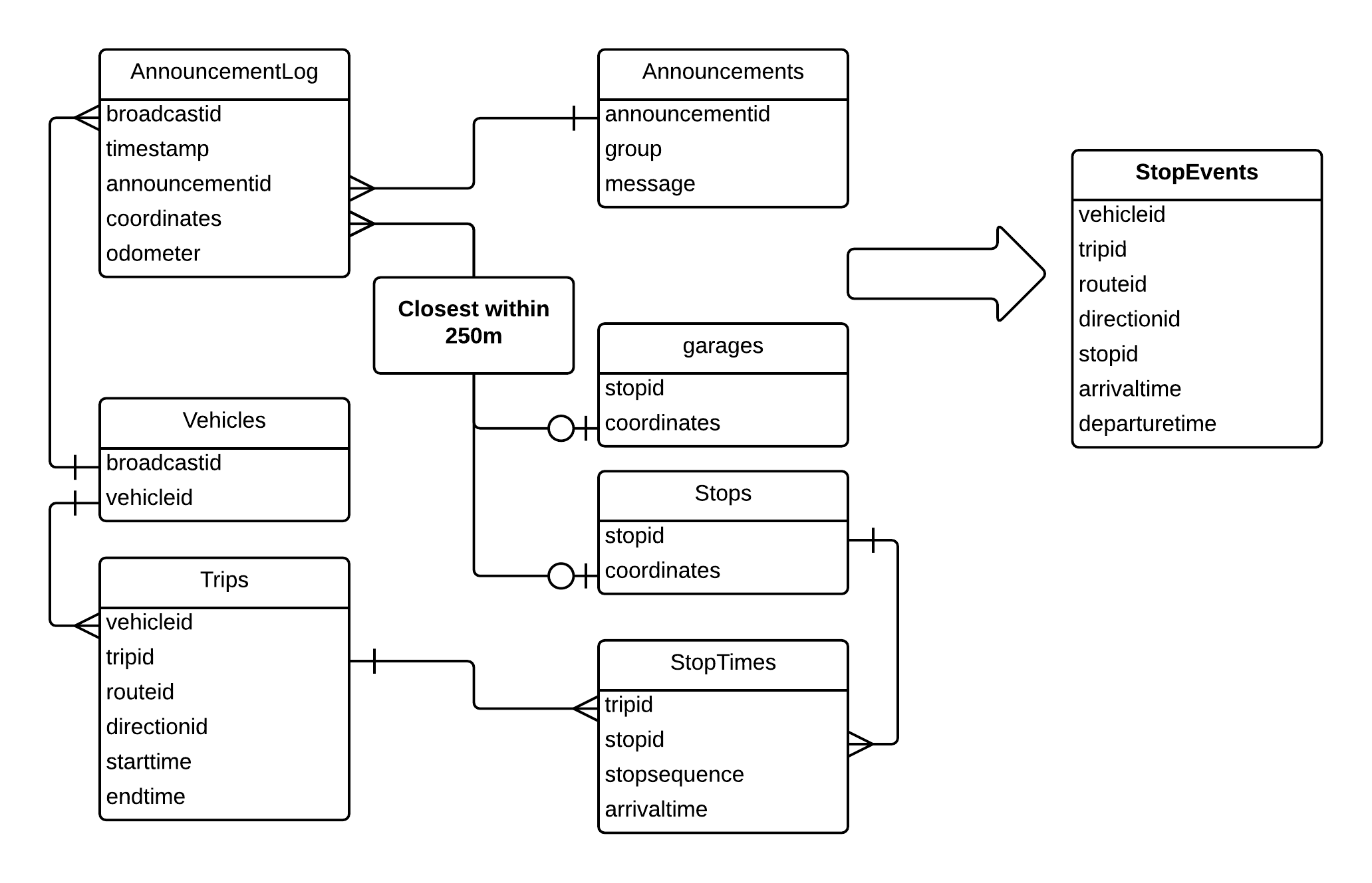
   Figure 2.8 Bus Announcement Entity Relationship Diagram for Processing Stop Events
2. Trip records are used to assign trips to external announcements based on their timestamps. The table is preprocessed to use observed arrival and departure values where possible, and also record the previous trip’s arrival and subsequent trip’s departure. This allows for temporal buffers of 15 minutes on trip start or end times while ensuring that these are not also joined to previous or subsequent trips.
3. The announcement log is joined to the announcement lookup table in order to use only external announcements. Geographic point objects are created using each announcement record’s latitude and longitude values. To prevent errors caused by invalid position values (outside [-90, 90] latitude, and [-180,180] longitude), a generous zone around Boston is used as a filter to ensure that GPS records are within the MBTA’s service area. The timestamp of each announcement record is compared to the pre-processed trip records.
4. For every external announcement, a k-nearest neighbors (k-NN) search is used to return the nearest stop either in the pattern for its assigned trip or the set of bus garages. If the bus was closer to a garage than to a stop along the pattern, that record is discarded. In order to remove erroneous GPS records or spurious events, those logged further than 250m (820ft) from the nearest stop were excluded.
5. In cases where stops appear out of sequence, odometer values (truncated to 1/10 mile or 160m) are used to determine whether this is due to an incorrect GPS record. If the distance between the snapped stop and the previous stop is greater than 400m (1312ft) the distance travelled according to the odometer the record is excluded. Other records that are out of order—for example if the bus is short-turned but this is not reflected in the vehicle trips table—are conserved.
6. The results from step 4 are joined to other tables to assign route, direction, stop name, stop sequence, and cumulative distance for each record.

The results for 21 weekdays yielded a median of 190,628 stop events served (standard deviation: 4,257), representing roughly 44 percent of scheduled service stops.

Low-Frequency, Regularly Recorded Positions

The buses also record and wirelessly transmit GPS position data to dispatchers and to published real-time feeds every 60 seconds[5]. Yang et al. (2013) describe a procedure to infer stop arrival times from these records using random sampling. This data source is the most reliable in terms of coverage of trips since positions are still broadcast and recorded when computer issues result in no announcements or timepoints being recorded.

Selection of Preferred Bus Location Data Source

Announcement records are clearly preferred over interpolating between timepoints because of the better resolution of the data source and the increased temporal accuracy. However, announcements records do not necessarily exist for every trip, and due to filtering of inaccurate GPS positions, records are excluded. It is possible to supplement these with fixed-interval GPS records, which are present in more trips. However there is valuable information in the announcement records not absent from the more frequent (every 60sec) records: notably whether the bus opened its doors (and therefore whether any passenger could have boarded or alighted). Having arrival times for all scheduled stops introduces false positives inferred at locations where buses did not actually stop. Therefore it was preferred to have a smaller set of AVL data, and therefore lower OD inference rate, with higher confidence in observed behavior. Thus the external announcement data set is used in this research.

Processing Behind-the-Gate Arrival Times

For modes in which customers have access to a network, rather than a single bus route, of stops and stations after paying their fares, a new arrival-time inference process was developed and is described in 2.5.2 below. The algorithm was designed to use GTFS stop times, in order to maximize portability of the code, to facilitate testing, and to be able to process lines (the Green Line LRT) which do not yet have stop-level vehicle tracking. The goal of this “behind-the-gate” data preprocessing algorithm was therefore to produce an equivalent set of stop times using observed data. This was done by combining data for the 3 different modes that can be accessed behind the gate as detailed in Table 2.2.

Table 2.2 Data Sources Used for Underground Arrival Times

Mode	Data Stream Used
LRT	GTFS scheduled stop arrival times
BRT	Processed external announcements (see the External Announcements heading of section 2.3.2 above)
Heavy Rail	Track circuit records

Heavy rail data come in the form of track circuit records on the three heavy rail lines, for which the processing algorithm is describe in the following paragraphs. Figure 2.9 below shows the different tables used in this processing, as well as the output of the processing algorithm.

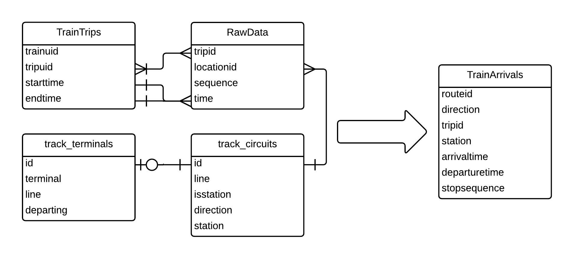
Figure 2.9 Track Processing Relational Diagram and Output Data

Each record contains a trip ID, a timestamp, and the location ID of that circuit. By matching location IDs to a lookup table, one can match records to their locations, and whether that circuit is at a station platform. There is one circuit per platform per direction.

Because of the use of multiple platforms at terminals, not all circuits are reliably triggered for station arrival and exit. A table was prepared of track circuits which are reliably triggered when trains enter or exit those terminal platforms. By filtering the circuit records for either being one of those terminal track circuits or presence at a station, the resulting set has platform arrival times for all stations and departure times at terminals. For arrival times in this set, the algorithm then finds an approximate departure time using the next triggered circuit. Since the goal of this processing was to provide data to determine the feasibility of an individual boarding a given train and then that train’s arrival time where the individual alighted, rather than determine accurate dwell times, this was deemed a satisfactory estimate of platform arrivals and departures.

On two branches, the trip IDs change to the subsequent ID prior to arriving at the terminal, between the penultimate station and the terminal. This is corrected for by using the previous trip ID as the trip ID if the previous station is different from the current record’s station. If the previous station is the same, then the train has reached a terminal and the trip ID will be different from the previous ID.

For the three heavy rail lines the output is an average of 17,581 stop events per Friday (SD=65) and 17,093 stop events per Monday-Thursday weekday (SD = 437) which is 94.4% of the scheduled Friday stops service and 96.1% of scheduled Monday-Thursday stops service.

Bus OD Inference

This was performed using the same process as in London (Gordon, 2012), with the Java code being updated to accept different input data. Because AFC transactions in Boston are precise to the second, origin inference was modified so that the origin of transactions are assigned to the stop immediately preceding the transaction time, except for a user-specified buffer before the next stop. In London, transactions were truncated to the minute, so transactions were assumed to occur on the 30^th second, and due to this imprecision in time, origins were assigned to the closest stop in time.

The sensitivity of destination-inference rates to user-specified parameters was compared between the two cities. The distance from the candidate alighting location to the user’s target destination (the subsequent origin or the first origin of the day) is graphed in Figure 2.10. The parameter was originally 750m however a second maximum in the distribution was discovered between 750m and 1000m. Increasing the maximum destination inference parameter to 1000m would result in a potential increase in destination inference rate of 2.1 percentage points.

Underground Destination and Arrival Time Inference

Unlike London’s closed rail system, which yields the times and locations of passenger origins and destinations, Boston’s underground rapid transit network, which allows behind-the-gate transfers, is an open fare payment system. Destination locations and times must therefore be inferred for Boston’s rapid transit lines (heavy rail, light rail, and bus rapid transit) which offer transfers underground. The methodology developed is described below.

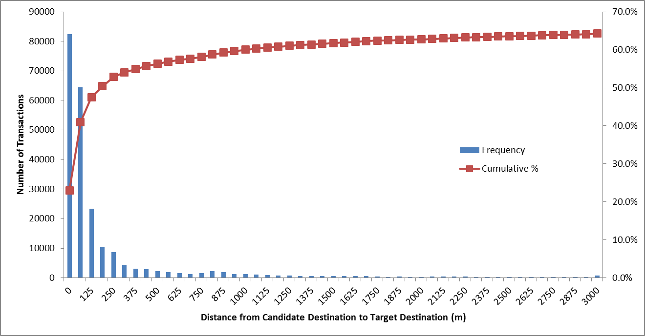
Figure 2.10 Comparing Sensitivity to Destination Inference Distance for Bus

Other examples of destination inference in rail networks

Barry et al. (2009), Munizaga and Palma (2012), and Zhao, Rahbee and Wilson (2007) all infer destination for open rail systems in New York City, Santiago de Chile, and Chicago respectively. All three methodologies use a nearest-stop assumption: that the user’s destination is closest to their subsequent transaction and that at the end of the day the user returns to their first origin.

To infer alighting times, Barry et al use a schedule-based shortest path algorithm to estimate an alighting time based on scheduled travel time. Munizaga and Palma use a shortest path algorithm based on AVL to infer alighting times at Metro station. Zhao et al do not infer arrival times.

Methodology

Destinations are inferred using the aforementioned nearest-stop assumption with the set of feasible destinations being every surface and subway stop and station in the rapid transit network (see Figure)[6]. Arrival times are then inferred using the following methodology.

Arrival Time Inference Procedure

The authors prepared a deterministic path matrix for all rail OD pairs which was stored in a database as arrays of segments (each segment representing travel between one boarding and alighting along a single line) where each row contained:

{Origin station, destination station, route, direction, alighting station, segment number}

The segment number increments from 1 for each segment required to go from origin to destination. The following assumptions were made:

• Customers board the earliest train that stops at their segment alighting location.
• Crowding does not prevent riders from boarding.
• Arrival-time data are complete.
• System wide access, egress, and transfer parameters are static.

The arrival-time inference algorithm is executed as follows (see Figure 2.11):

1. Look up the path for an inferred passenger OD pair.
2. For each segment:
   1. Find the first trip to arrive after the customer’s transaction, for the specified origin station, line, and direction.
   2. Find that vehicle’s arrival time at the alighting station.
   3. If there is no arrival time, return to 2.a.
3. If the segment sequence number is equivalent to the size of the path array then the alighting station is the destination and the arrival time is recorded. Otherwise use the alighting station as the next boarding station and the alighting station arrival time as the new transaction time and repeat from 2.a.

Arrival inference was initially tested using GTFS scheduled data, and then a hybrid of track data (where available) and schedule data was used. The number of successfully inferred rail destinations increased by 4,300 (0.9%) using track circuit data versus simply using schedule data because these customers were inferred to arrive in time to board their next bus. Many of these passenger trips were then inferred to have been linked to the customer’s previous or subsequent bus or rail trips.

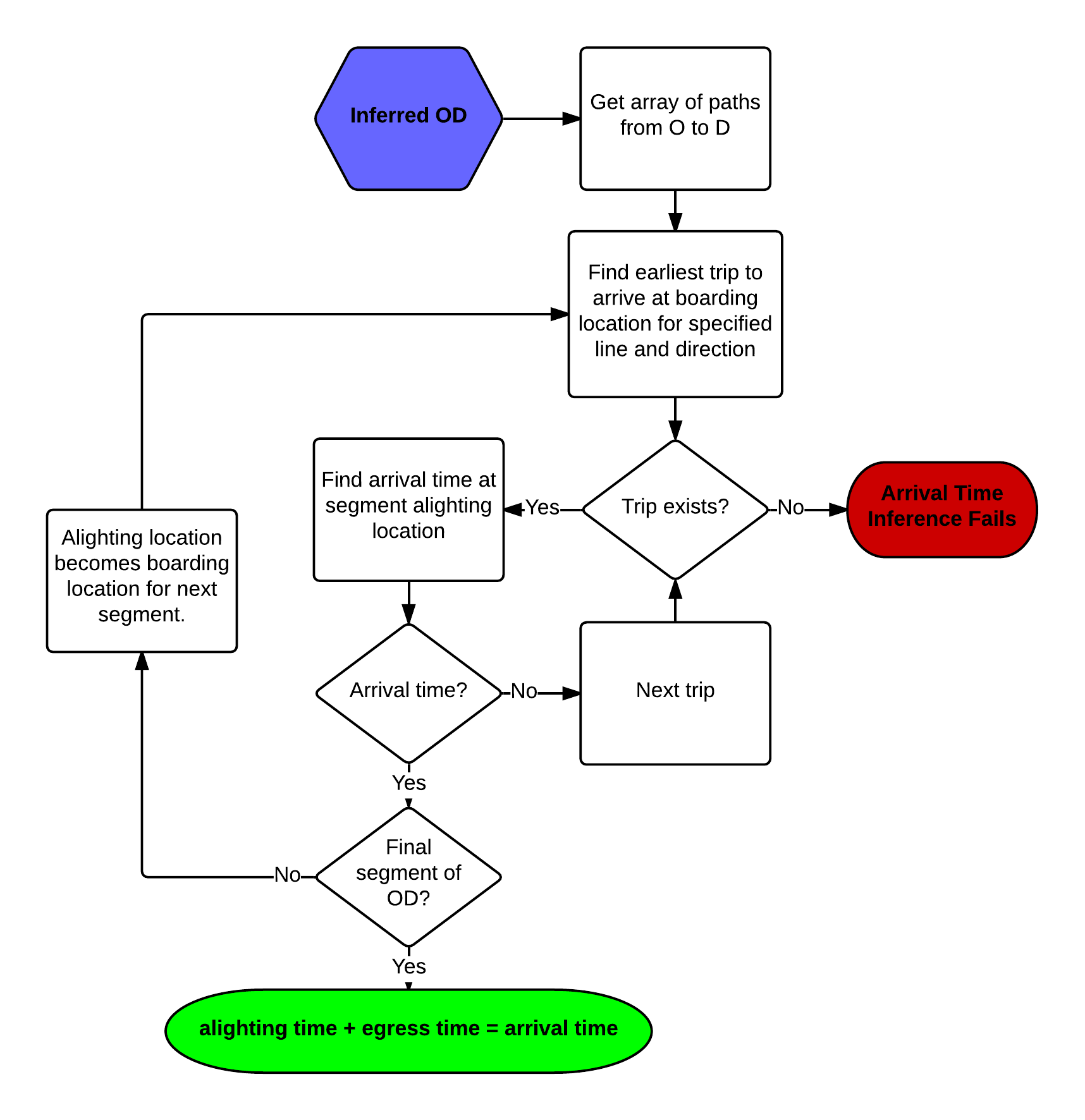
Figure 2.11 Arrival Time Inference Flow Chart

Interchange Inference

The same process as performed in London was used (Gordon, 2012) with the following parameters:

• Minimum walk speed = 3000 m/hr
• Maximum transfer distance = 1000 meters
• Maximum bus wait time = 45 minutes
• Minimum transfer time allowance = 5 minutes
• Circuity factor = 1.7
• Minimum linked journey distance = 400 meters

The sensitivity of each parameter was compared between Boston and London. No significant differences in user behavior were observed, so the parameters remained unchanged. See Appendix A for this sensitivity testing. Overall 12.6% of weekday stages are linked into multi-stage journeys. Due to the conservative setting of parameters, the inference rate is likely lower than the true rate of journey linking. Inferred transfer rates are below those estimated by the Central Transportation Planning Staff from surveys (Vanderwaart, 2015) and testing of the inference procedure is ongoing.

Table 2.3 shows the proportion of stage-pairs that could be linked and that are linked by the combination of lines and mode used. The second column indicates the total number of sets of the stage-pair in the first column which occurred on weekdays in April 2014 and the table is sorted in descending order on the third column: the stage-pairs which were successfully linked into journeys. Stages were classified by their originating mode or line, in the case of rail. The following were excluded:

• Stages where the subsequent stage was on the same route, or heavy rail after a heavy rail stage, since all heavy rail interchanges would happen behind the gate
• Stages for customers who only had one stage on a given day, including stages where cash was used, since there are no subsequent stages to link the current stage to
• Final stages of the day, since there are no subsequent stages to link the current stage to on that day
• Stage-pairs that included an origin on the surface portion of the Green Line, since due to the lack of origin coordinates and stage travel times, it is impossible to link these

Examining the absolute numbers of linked journeys, one immediately notices an asymmetry between bus and any subway line: overall, fewer journeys are linked where a user transfers from bus to rail than the reverse. However, this asymmetry also appears in the number in the second column, fewer users travel from bus to rail subsequently than the converse, especially for the Orange and Red Lines. Anecdotal evidence suggests this may due to bus drivers waving on users with passes where the pass validity is printed on the ticket due to large volumes of users boarding from the subway to the bus. This would lead to fewer bus boardings being recorded by the AFC system at heavy rail stations, and consequently fewer observed “heavy rail> bus” pairs of stages being recorded. The second to last column, which shows the ratio between the rail-to-bus linked stages versus bus-to-rail shows only a small discrepancy in the link rates for the Orange and Red Lines.

Table 2.3 Potentially Linked Transfer Pairs of Stages and Transfer Rates

Stage->Next Stage	Potential Linked Stage-Pairs	Linked Stage-Pairs	Link Rate	Destination Inference Rate	Arrival Time Inference Rate	Rail-bus Ratio	Ratio of Arrival Time Inference
bus->bus	2,323,510	515,717	22.2%	73.0%	73.0%
Bus->Orange Line	722,700	473,103	65.5%	79.9%	79.9%
bus->Red Line	670,395	361,009	53.9%	74.4%	74.4%
Red Line->bus	659,817	341,483	51.8%	77.3%	70.0%	96.1%	94.1%
Orange Line->bus	634,678	383,172	60.4%	80.0%	76.1%	92.2%	95.2%
bus->Green Line	138,472	67,712	48.9%	75.7%	75.7%
Green Line->bus	126,393	51,736	40.9%	75.6%	55.1%	83.7%	72.8%
Bus->Blue Line	119,881	72,608	60.6%	75.7%	75.7%	65.6%	69.2%
Blue Line->bus	101,992	40,543	39.8%	76.9%	52.4%
Bus->Silver Line	2,046	50	2.4%	40.9%	40.9%

This column shows a different story for the Green and Blue lines, the difference in linking rates is more significant. This appears to be due to an asymmetry in arrival time inference. While destinations tend to be inferred at a higher rate on heavy rail, arrival times are not being inferred at a rate similar to the Orange and Red Lines on these two rail lines. This is currently being investigated and will be improved upon in future versions of ODX.

Processing Months of Data

The goal of the OD inference module is to run the algorithm one day at a time, once all the necessary inputs have been assembled. For retrospective analysis, however, it was necessary to infer OD for months of data at once. The AFC and AVL preprocessing scripts were programmed as PostgreSQL functions which could be queried to run over multiple days. A Bash script was developed which prepares the parameter file, calls the Java OD-inference algorithm, and then runs a COPY command to upload the results to a database. Performing OD inference for a month required approximately 30 minutes for the full MBTA system on a Linux server with a 6 core, 12 thread CPU at 3.2GHz and 64GB of 1333 MHz RAM.

Results and Validation

Table 2.4 below shows the inference rates by mode for all weekdays in April 2014 and the top 5 sources of destination inference failure. Because of the lack of AVL on the LRT, origin and destination inference is at a branch level on surface LRT branches. The top 2 main contributors to destination inference failure are:

1. Users who only make one transaction per day, and
2. Users’ target destination being the same location as their current origin

In either case, there is insufficient information for that day from which a destination can be inferred. The latter case is partially due to the ability for users’ to gain entry for multiple people on a single card or ticket using Stored Value.

Destination inference is higher on the rail modes over the bus modes since rail users tend to use rail for the stage (either the subsequent stage, or the first of the day) that determines their target destination. For rail stages with the target destination at a rail station, the distance between a user’s inferred destination and the target is 0, since the destination will be inferred to be at the closest station to the target destination station which are one and the same. It is therefore likely that false positive inferences are introduced for these modes, since a user who uses a non-transit mode between rail stages can still have their destination inferred, since the destination distance and the travel direction tests do not apply to this case. This is less the case on bus, since each route is a distinct line, and therefore users using non-transit modes between stages are likely to travel more than the maximum destination inference distance of 1000m between bus routes, or travel in a manner to make the direction test fail.

Table 2.4 Inference Rates by Mode

	Bus	Surface LRT	Heavy Rail
Origin Inference	97.1%	100%	100%
Destination Inference	56.4%	77.0%	74.8%
Only One Stage In a Day	8.72%	16.7%	14.9%
Distance Greater than 1000m	8.80%	2.10%	3.70%
Target Destination same as Current Origin	7.23%	0%	4.69%
Cash	5.21%	3.50%	0%
User Travelling Away from Target Destination	4.77%	0.%	0%

Table 2.5 lists the top 10 routes by destination inference rate for April 2014 weekdays and Table 2.6 lists the bottom 10 routes by destination inference rate. For comparison the route with the highest ridership, the 66, had nearly 11,500 daily riders, and the 32 has the eighth-highest ridership. Routes with higher destination inference tend to have more ridership but don’t necessarily have higher origin inference. These routes are clustered around the Orange Line in the South West or serving the Orange and Red Lines from the North.

Of the routes with low destination inference, the routes with IDs like 4XX are geographically clustered around Lynn or Salem, to the North East of Boston. The 7XX routes are the surface portions of the Silver Line BRT, and their low inference is due to the algorithm not yet processing destinations within the rapid transit network from surface bus origins.

Table 2.5 Bus Routes with the Highest Destination Inference Rates

Route	Origin Inference Rate	Destination Inference Rate	Average Daily Ridership
132	98.2%	66.9%	799
50	97.9%	66.7%	1,108
352	99.3%	66.6%	272
428	100.0%	66.1%	127
87	98.6%	65.9%	3,262
701	96.5%	65.6%	2,035
97	99.6%	65.6%	856
32	97.1%	65.5%	8,468
106	98.1%	65.1%	2,457
45	97.9%	64.6%	2,590

Table 2.6 Bus Routes with the Lowest Destination Inference Rate

Route	Origin Inference Rate	Destination Inference Rate	Average Daily Ridership
431	40.1%	0.3%	55
741	87.4%	11.7%	324
171	93.1%	18.6%	17
746	92.8%	21.8%	225
742	98.7%	21.9%	1,100
465	96.7%	24.8%	310
451	99.9%	31.1%	130
429	99.4%	33.7%	1,283
436	99.4%	34.2%	632
52	96.3%	34.9%	523
435	99.9%	35.3%	720

The chart in Figure 2.12 shows the distribution of the number of stages for weekday journeys over the month. The mode is the mode of the first stage of the journey. 100% of LRT journeys are single stage since there is insufficient information (origin coordinates and time), for interchange inference to occur. Nearly 25% of bus journeys involve more than one stage whereas fewer than 10% of heavy rail journeys do (this does not include behind the gate transfers).

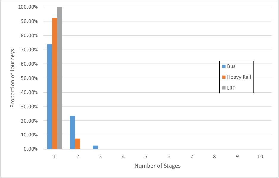
Figure 2.12 Stage Distribution by Mode

Validation

The results of bus OD inference was previously validated in London comparing the stage distribution to the London Travel Demand Survey (LTDS) (Gordon, 2012). No external data source which provided OD flows over the processed time period was available for large-scale validation of inference with the MBTA data. Load profiles were created for bus routes for visual inspection of results and the inference rate per route was analyzed to determine outlier routes. Additional validation is ongoing through the examination of bus loads and comparison with APC data. Subsequent to these validation exercises, the existing OD inference procedure may be improved in the future.

Summary

The methods originally developed to infer bus origins and destinations and multimodal interchanges in the London network (Gordon, 2012) have been updated to infer origins and destinations on the fully open multimodal system of the MBTA. Though the results of the OD inference algorithm have not been tested at large scale, there is evidence that estimates are reasonable. Scripts have been used to infer months of OD from archived data, and this output is further processed by a methodology described in Chapter 4 to generate performance metrics for the purpose of analyzing the spatial variation of transit travel described in Chapter 5.